


What is a neural network?
A neural network is just a mathematical function, which contains some layers.
"No Worries we will discuss more about layers in this blog"
Let's Consider a simple function that does :
Multiplies each input by several values. These values are known as parameters
Adds them up for each group of values
Replaces the negative numbers with zeros
This represents one "layer". Then these three steps are repeated, using the outputs of the previous layer as the inputs to the next layer. Initially, the parameters in this function are selected randomly. Therefore a newly created neural network doesn't do anything useful at all -- it's just random!
How do neural networks work?
To get the function to learn to do something useful, we have to change the parameters to make them better in some way. We do this using gradient descent. Let's see how this works...
"No worries we see all these fascinating words (Highlighted one) in detail"
Gradient Descent - How it works?
Before coming to the definition part of What is Gradient Descent? Let's first see How and what it works?
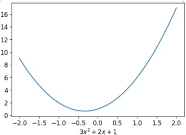
To learn how gradient descent works, Let's take a quadratic function and try to fit it since that's a function most of us are probably more familiar with than a neural network. Here's the quadratic we're going to try to fit:
def f(x): return 3*x**2 + 2*x + 1 #defining the quadratic function

plot_function(f, "$3x^2 + 2x + 1$")
It plots the graph of this quadratic function, Here we go
Now Let's generalise the whole Quadratic function
def quad(a, b, c, x): return a*x**2 + b*x + c
def mk_quad(a,b,c): return partial(quad, a,b,c)
If we fix some particular values of a, b, and c, then we'll have made a quadratic. To fix values passed to a function in Python, we use the partial function
f2 = mk_quad(3,2,1)
plot_function(f2)
Same output as the previous one as we generate the same quadratic function
Now, in the real world, the data is not straightforward like this function it has some noise, so I am going to create some noisy data
def noise(x, scale): return np.random.normal(scale=scale, size=x.shape)
def add_noise(x, mult, add): return x * (1+noise(x,mult)) + noise(x,add)
These functions put noise in our data, the noise here basically means that our y didn't the same as in the case of previously generated quadratic function for the same X
np.random.seed(42)

x = torch.linspace(-2, 2, steps=20)[:,None]
y = add_noise(f(x), 0.15, 1.5)

plt.scatter(x,y);
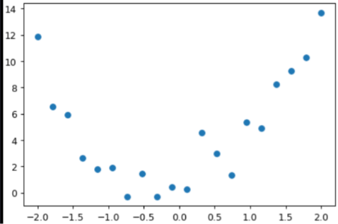
It's not the quadratic function that we have created, So our challenge is to find the function which fits this data. In other words, we have to find the new a,b, and c for which this data will fit more accurately
For this, we have some options
Manually change the value of a,b and c
Use Calculus to figure out a,b and c
and observe the change in the graph by plotting it and try to find the most appropriate value of a,b and c
Manual approach
@interact(a=1.1, b=1.1, c=1.1)
def plot_quad(a, b, c):
    plt.scatter(x,y)
    plot_function(mk_quad(a,b,c), ylim=(-3,13))
Here's a function that overlays a quadratic on top of our data, along with some sliders to change a, b, and c, and see how it looks:

Try moving slider a bit to the left. Does that look better or worse? How about if you move it a bit to the right? Find out which direction seems to improve the fit of the quadratic to the data, and move the slider a bit in that direction. Next, do the same for slider b: first figure out which direction improves the fit, then move it a bit in that direction. Then do the same for c and repeat the same.
One thing that's making this tricky is that we don't really have a great sense of whether our fit is really better or worse. It would be easier if we had a numeric measure of that. An easy metric we could use is a mean absolute error -- which is the distance from each data point to the curve:
def mae(preds, acts): return (torch.abs(preds-acts)).mean()
# mae -> Mean absolute error
@interact(a=1.5, b=1.5, c=1.5)
def plot_quad(a, b, c):
    f = mk_quad(a,b,c)
    plt.scatter(x,y)
    loss = mae(f(x), y)
    plot_function(f, ylim=(-3,12), title=f"loss: {loss:.2f}")
Here we go
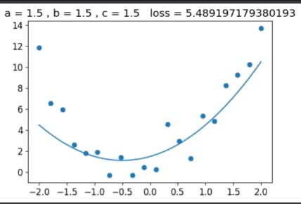
Example after changing the "a" we notice that loss decreased
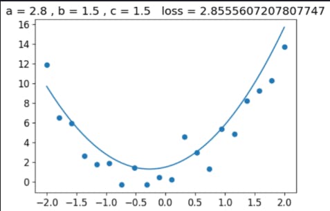
Do this similarly until u minimised your loss in your system to get the better visualization
In a modern neural network, we'll often have tens of millions of parameters(Here it's a,b and c) to fit or more, and thousands or millions of data points to fit them. We're not going to be able to do that by moving sliders around! We'll need to automate this process.
Calculus approach
Uh oh, calculus! If you haven't touched calculus since school, you might be getting ready to run away at this point. But don't worry, we don't actually need much calculus at all. Just derivatives, which measure the rate of change of a function. We don't even need to calculate them ourselves, because the computer will do it for us!
Automating Gradient Descent
If you are thinking that Gradient Descent came Suddenly after a long go , so, Now it's Time to Understand what Gradient Descent Does :
Think, When you are increasing or decreasing the parameters we have seen previously by adjusting the Slider, what we are logically doing is that we are adding or subtracting some constant in that parameters for decreasing the mae() ,that constant is known as Gradient if we are considering the learning rate as 1
Again some fancy words like "learning rate", but no worries we will discuss the concept of learning rate in some other blog
So in a broader sense, we can say that a Gradient Descent is a concept for calculating gradient, but u may think that how it's calculated ?
Ya well it's another deep concept that how gradients are calculated we will surely cover in another blog but if u didn't want to wait for it just go through the concept of BackPropogation
Returning back to the topic of automating Gradient Descent
The basic idea is this: if we know the gradient of our mae() function with respect to our parameters, a, b, and c, then that means we know how to adjust (for instance) a will change the value of mae(). If, say, a has a negative gradient, then we know that increasing a will decrease mae(). Then we know that's what we need to do since we trying to make mae() as low as possible.
So, we find the gradient of mae() for each of our parameters, and then adjust our parameters a bit in the opposite direction to the sign of the gradient.
To do this, first, we need a function that takes all the parameters a, b, and c as a single vector input, and returns the value mae() based on those parameters:
Here we go
def quad_mae(params):
    f = mk_quad(*params)
    return mae(f(x), y)
We're first going to do exactly the same thing as we did manually -- pick some arbitrary starting point for our parameters. We'll put them all into a single tensor:
abc = torch.tensor([1.1,1.1,1.1])
To tell PyTorch that we want it to calculate gradients for these parameters, we need to call requires_grad_():
abc.requires_grad_()
We can now calculate mae(). Generally, when doing gradient descent, the thing we're trying to minimise is called the loss:
loss = quad_mae(abc)
loss

To get PyTorch to now calculate the gradients, we need to call backward()
loss.backward()
The gradients will be stored for us in an attribute called grad:
abc.grad

According to these gradients, all our parameters are a little low. So let's increase them a bit. If we subtract the gradient, multiplied by a small number(this small number is the learning rate), that should improve them a bit:
The above gradient just simply means that if we have to decrease the loss more efficiently we have to increase parameter "a" the most then "c" and "b"
with torch.no_grad():
    abc -= abc.grad*0.01
    loss = quad_mae(abc)

print(f'loss={loss:.2f}')
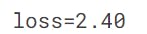
ye! We decrease our loss
BTW, you'll see we had to wrap our calculation of the new parameters in with torch.no_grad(). That disables the calculation of gradients for any operations inside that context manager. We have to do that, because abc -= abc.grad*0.01 isn't actually part of our quadratic model, so we don't want derivitives to include that calculation.
I know this above line may be tough to understand for some guys but when I publish my back propagation blog I dig deeper into it
We can use a loop to do a few more iterations of this:
for i in range(10):
    loss = quad_mae(abc)
    loss.backward()
    with torch.no_grad(): abc -= abc.grad*0.01
    print(f'step={i}; loss={loss:.2f}')
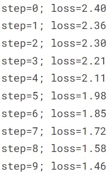
As you can see, our loss keeps going down!
If you keep running this loop for long enough, however, you'll see that the loss eventually starts increasing for a while. That's because once the parameters get close to the correct answer, our parameter updates will jump right over the correct answer! To avoid this, we need to decrease our learning rate as we train. This is done using a learning rate schedule and can be automated in most deep learning frameworks, such as PyTorch as well as fastai.
and once u get the parameter that is close to the correct answer for some particular input our model gets trained and that's how the neural network works.